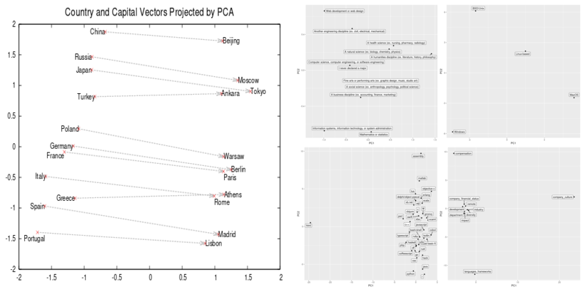
What’s helpful about embeddings? Relying on who you ask, solutions could fluctuate. For a lot of, essentially the most instant affiliation could also be phrase vectors and their use in pure language processing (translation, summarization, query answering and so forth.) There, they’re well-known for modeling semantic and syntactic relationships, as exemplified by this diagram present in one of the crucial influential papers on phrase vectors(Mikolov et al. 2013):

Others will most likely deliver up entity embeddings, the magic device that helped win the Rossmann competitors(Guo and Berkhahn 2016) and was tremendously popularized by quick.ai’s deep studying course. Right here, the concept is to make use of knowledge that’s not usually useful in prediction, like high-dimensional categorical variables.
One other (associated) concept, additionally extensively unfold by quick.ai and defined in this weblog, is to use embeddings to collaborative filtering. This principally builds up entity embeddings of customers and gadgets primarily based on the criterion how properly these “match” (as indicated by present scores).
So what are embeddings good for? The best way we see it, embeddings are what you make of them. The objective on this submit is to offer examples of learn how to use embeddings to uncover relationships and enhance prediction. The examples are simply that – examples, chosen to display a technique. Probably the most attention-grabbing factor actually might be what you make of those strategies in your space of labor or curiosity.
Embeddings for enjoyable (picturing relationships)
Our first instance will stress the “enjoyable” half, but in addition present learn how to technically take care of categorical variables in a dataset.
We’ll take this 12 months’s StackOverflow developer survey as a foundation and choose a number of categorical variables that appear attention-grabbing – stuff like “what do folks worth in a job” and naturally, what languages and OSes do folks use. Don’t take this too severely, it’s meant to be enjoyable and display a technique, that’s all.
Getting ready the info
Geared up with the libraries we’ll want:
We load the info and zoom in on a number of categorical variables. Two of them we intend to make use of as targets: EthicsChoice and JobSatisfaction. EthicsChoice is one in all 4 ethics-related questions and goes
“Think about that you simply have been requested to put in writing code for a function or product that you simply contemplate extraordinarily unethical. Do you write the code anyway?”
With questions like this, it’s by no means clear what portion of a response ought to be attributed to social desirability – this query appeared just like the least vulnerable to that, which is why we selected it.
information <- read_csv("survey_results_public.csv")

information <- information %>% choose(
  FormalEducation,
  UndergradMajor,
  starts_with("AssessJob"),
  EthicsChoice,
  LanguageWorkedWith,
  OperatingSystem,
  EthicsChoice,
  JobSatisfaction
)

information <- information %>% mutate_if(is.character, issue)
The variables we’re all for present a bent to have been left unanswered by fairly a number of respondents, so the simplest solution to deal with lacking information right here is to exclude the respective individuals fully.
That leaves us with ~48,000 accomplished (so far as we’re involved) questionnaires.
Wanting on the variables’ contents, we see we’ll need to do one thing with them earlier than we will begin coaching.
Observations: 48,610
Variables: 16
$ FormalEducation    <fct> Bachelor’s diploma (BA, BS, B.Eng., and so forth.),...
$ UndergradMajor     <fct> Arithmetic or statistics, A pure scie...
$ AssessJob1         <int> 10, 1, 8, 8, 5, 6, 6, 6, 9, 7, 3, 1, 6, 7...
$ AssessJob2         <int> 7, 7, 5, 5, 3, 5, 3, 9, 4, 4, 9, 7, 7, 10...
$ AssessJob3         <int> 8, 10, 7, 4, 9, 4, 7, 2, 10, 10, 10, 6, 1...
$ AssessJob4         <int> 1, 8, 1, 9, 4, 2, 4, 4, 3, 2, 6, 10, 4, 1...
$ AssessJob5         <int> 2, 2, 2, 1, 1, 7, 1, 3, 1, 1, 8, 9, 2, 4,...
$ AssessJob6         <int> 5, 5, 6, 3, 8, 8, 5, 5, 6, 5, 7, 4, 5, 5,...
$ AssessJob7         <int> 3, 4, 4, 6, 2, 10, 10, 8, 5, 3, 1, 2, 3, ...
$ AssessJob8         <int> 4, 3, 3, 2, 7, 1, 8, 7, 2, 6, 2, 3, 1, 3,...
$ AssessJob9         <int> 9, 6, 10, 10, 10, 9, 9, 10, 7, 9, 4, 8, 9...
$ AssessJob10        <int> 6, 9, 9, 7, 6, 3, 2, 1, 8, 8, 5, 5, 8, 9,...
$ EthicsChoice       <fct> No, Relies on what it's, No, Relies on...
$ LanguageWorkedWith <fct> JavaScript;Python;HTML;CSS, JavaScript;Py...
$ OperatingSystem    <fct> Linux-based, Linux-based, Home windows, Linux-...
$ JobSatisfaction    <fct> Extraordinarily glad, Reasonably dissatisf...
Goal variables
We need to binarize each goal variables. Let’s examine them, beginning with EthicsChoice.
jslevels <- ranges(information$JobSatisfaction)
elevels <- ranges(information$EthicsChoice)

information <- information %>% mutate(
  JobSatisfaction = JobSatisfaction %>% fct_relevel(
    jslevels[1],
    jslevels[3],
    jslevels[6],
    jslevels[5],
    jslevels[7],
    jslevels[4],
    jslevels[2]
  ),
  EthicsChoice = EthicsChoice %>% fct_relevel(
    elevels[2],
    elevels[1],
    elevels[3]
  )
)

ggplot(information, aes(EthicsChoice)) + geom_bar()
You may agree that with a query containing the phrase a function or product that you simply contemplate extraordinarily unethical, the reply “is dependent upon what it’s” feels nearer to “sure” than to “no.” If that looks like too skeptical a thought, it’s nonetheless the one binarization that achieves a smart break up.
Taking a look at our second goal variable, JobSatisfaction:

We predict that given the mode at “reasonably glad,” a smart solution to binarize is a break up into “reasonably glad” and “extraordinarily glad” on one facet, all remaining choices on the opposite:
Predictors
Among the many predictors, FormalEducation, UndergradMajor and OperatingSystem look fairly innocent – we already turned them into elements so it ought to be easy to one-hot-encode them. For curiosity’s sake, let’s take a look at how they’re distributed:
  FormalEducation                                        depend
  <fct>                                                  <int>
1 Bachelor’s diploma (BA, BS, B.Eng., and so forth.)               25558
2 Grasp’s diploma (MA, MS, M.Eng., MBA, and so forth.)            12865
3 Some faculty/college research with out incomes a level  6474
4 Affiliate diploma                                        1595
5 Different doctoral diploma (Ph.D, Ed.D., and so forth.)               1395
6 Skilled diploma (JD, MD, and so forth.)                       723
UndergradMajor depend
<fct> <int>
1 Laptop science, pc engineering, or software program engineering 30931
2 One other engineering self-discipline (ex. civil, electrical, mechani… 4179
3 Info methods, info expertise, or system adminis… 3953
4 A pure science (ex. biology, chemistry, physics) 2046
5 Arithmetic or statistics 1853
6 Internet growth or net design 1171
7 A enterprise self-discipline (ex. accounting, finance, advertising) 1166
8 A humanities self-discipline (ex. literature, historical past, philosophy) 1104
9 A social science (ex. anthropology, psychology, political scie… 888
10 Wonderful arts or performing arts (ex. graphic design, music, studi… 791
11 I by no means declared a significant 398
12 A well being science (ex. nursing, pharmacy, radiology) 130 OperatingSystem depend
<fct> <int>
1 Home windows 23470
2 MacOS 14216
3 Linux-based 10837
4 BSD/Unix 87LanguageWorkedWith, alternatively, incorporates sequences of programming languages, concatenated by semicolon.
One solution to unpack these is utilizing Keras’ text_tokenizer.
language_tokenizer <- text_tokenizer(break up = ";", filters = "")
language_tokenizer %>% fit_text_tokenizer(information$LanguageWorkedWith)
We’ve got 38 languages total. Precise utilization counts aren’t too shocking:
                   title depend
1            javascript 35224
2                  html 33287
3                   css 31744
4                   sql 29217
5                  java 21503
6            bash/shell 20997
7                python 18623
8                    c# 17604
9                   php 13843
10                  c++ 10846
11           typescript  9551
12                    c  9297
13                 ruby  5352
14                swift  4014
15                   go  3784
16          objective-c  3651
17               vb.web  3217
18                    r  3049
19             meeting  2699
20               groovy  2541
21                scala  2475
22               matlab  2465
23               kotlin  2305
24                  vba  2298
25                 perl  2164
26       visible fundamental 6  1729
27         coffeescript  1711
28                  lua  1556
29 delphi/object pascal  1174
30                 rust  1132
31              haskell  1058
32                   f#   764
33              clojure   696
34               erlang   560
35                cobol   317
36                ocaml   216
37                julia   215
38                 hack    94
Now language_tokenizer will properly create a one-hot illustration of the multiple-choice column.
langs <- language_tokenizer %>%
  texts_to_matrix(information$LanguageWorkedWith, mode = "depend")
langs[1:3, ]
> langs[1:3, ]
[,1] [,2] [,3] [,4] [,5] [,6] [,7] [,8] [,9] [,10] [,11] [,12] [,13] [,14] [,15] [,16] [,17] [,18] [,19] [,20] [,21]
[1,] 0 1 1 1 0 0 0 1 0 0 0 0 0 0 0 0 0 0 0 0 0
[2,] 0 1 0 0 0 0 1 1 0 0 0 0 0 0 0 0 0 0 0 0 0
[3,] 0 0 0 0 1 1 1 0 0 0 1 0 1 0 0 0 0 0 1 0 0
[,22] [,23] [,24] [,25] [,26] [,27] [,28] [,29] [,30] [,31] [,32] [,33] [,34] [,35] [,36] [,37] [,38] [,39]
[1,] 0 0 0 0 0 0 0 0 0 0 0 0 0 0 0 0 0 0
[2,] 0 0 0 0 0 0 0 0 0 0 0 0 0 0 0 0 0 0
[3,] 0 1 0 0 0 0 0 0 0 0 0 0 0 0 0 0 0 0We are able to merely append these columns to the dataframe (and do some cleanup):
We nonetheless have the AssessJob[n] columns to take care of. Right here, StackOverflow had folks rank what’s necessary to them a few job. These are the options that have been to be ranked:
The trade that I’d be working in
The monetary efficiency or funding standing of the corporate or group
The particular division or group I’d be engaged on
The languages, frameworks, and different applied sciences I’d be working with
The compensation and advantages supplied
The workplace atmosphere or firm tradition
The chance to work at home/remotely
Alternatives for skilled growth
The range of the corporate or group
How extensively used or impactful the services or products I’d be engaged on is
Columns AssessJob1 to AssessJob10 comprise the respective ranks, that’s, values between 1 and 10.
Primarily based on introspection concerning the cognitive effort to truly set up an order amongst 10 gadgets, we determined to drag out the three top-ranked options per individual and deal with them as equal. Technically, a primary step extracts and concatenate these, yielding an middleman results of e.g.
$ job_vals<fct> languages_frameworks;compensation;distant, trade;compensation;growth, languages_frameworks;compensation;growthinformation <- information %>% mutate(
val_1 = if_else(
AssessJob1 == 1, "trade", if_else(
AssessJob2 == 1, "company_financial_status", if_else(
AssessJob3 == 1, "division", if_else(
AssessJob4 == 1, "languages_frameworks", if_else(
AssessJob5 == 1, "compensation", if_else(
AssessJob6 == 1, "company_culture", if_else(
AssessJob7 == 1, "distant", if_else(
AssessJob8 == 1, "growth", if_else(
AssessJob10 == 1, "range", "affect"))))))))),
val_2 = if_else(
AssessJob1 == 2, "trade", if_else(
AssessJob2 == 2, "company_financial_status", if_else(
AssessJob3 == 2, "division", if_else(
AssessJob4 == 2, "languages_frameworks", if_else(
AssessJob5 == 2, "compensation", if_else(
AssessJob6 == 2, "company_culture", if_else(
AssessJob7 == 1, "distant", if_else(
AssessJob8 == 1, "growth", if_else(
AssessJob10 == 1, "range", "affect"))))))))),
val_3 = if_else(
AssessJob1 == 3, "trade", if_else(
AssessJob2 == 3, "company_financial_status", if_else(
AssessJob3 == 3, "division", if_else(
AssessJob4 == 3, "languages_frameworks", if_else(
AssessJob5 == 3, "compensation", if_else(
AssessJob6 == 3, "company_culture", if_else(
AssessJob7 == 3, "distant", if_else(
AssessJob8 == 3, "growth", if_else(
AssessJob10 == 3, "range", "affect")))))))))
)
information <- information %>% mutate(
job_vals = paste(val_1, val_2, val_3, sep = ";") %>% issue()
)
information <- information %>% choose(
-c(starts_with("AssessJob"), starts_with("val_"))
)Now that column appears precisely like LanguageWorkedWith regarded earlier than, so we will use the identical technique as above to provide a one-hot-encoded model.
values_tokenizer <- text_tokenizer(break up = ";", filters = "")
values_tokenizer %>% fit_text_tokenizer(information$job_vals)
So what really do respondents worth most?
                      title depend
1              compensation 27020
2      languages_frameworks 24216
3           company_culture 20432
4               growth 15981
5                    affect 14869
6                division 10452
7                    distant 10396
8                  trade  8294
9                 range  7594
10 company_financial_status  6576
Utilizing the identical technique as above
we find yourself with a dataset that appears like this
> information %>% glimpse()
Observations: 48,610
Variables: 53
$ FormalEducation          <fct> Bachelor’s diploma (BA, BS, B.Eng., and so forth.), Bach...
$ UndergradMajor           <fct> Arithmetic or statistics, A pure science (...
$ OperatingSystem          <fct> Linux-based, Linux-based, Home windows, Linux-based...
$ JS                       <dbl> 1, 0, 0, 1, 0, 0, 1, 1, 1, 0, 0, 0, 1, 1, 0, 0...
$ EC                       <dbl> 0, 1, 0, 1, 1, 1, 0, 1, 0, 0, 0, 0, 0, 1, 0, 0...
$ javascript               <dbl> 1, 1, 0, 1, 1, 1, 1, 0, 0, 0, 1, 1, 1, 1, 0, 1...
$ html                     <dbl> 1, 0, 0, 1, 1, 1, 1, 0, 1, 0, 1, 1, 1, 1, 1, 1...
$ css                      <dbl> 1, 0, 0, 1, 1, 1, 1, 0, 1, 0, 1, 1, 1, 1, 0, 1...
$ sql                      <dbl> 0, 0, 1, 0, 0, 0, 1, 0, 1, 1, 1, 1, 1, 1, 1, 1...
$ java                     <dbl> 0, 0, 1, 1, 0, 0, 0, 1, 0, 0, 0, 1, 1, 0, 0, 1...
$ `bash/shell`             <dbl> 0, 1, 1, 0, 0, 0, 1, 0, 1, 0, 0, 0, 0, 0, 1, 1...
$ python                   <dbl> 1, 1, 0, 1, 0, 0, 1, 0, 0, 1, 0, 0, 0, 0, 1, 0...
$ `c#`                     <dbl> 0, 0, 0, 0, 0, 0, 0, 0, 1, 0, 1, 0, 1, 1, 0, 0...
$ php                      <dbl> 0, 0, 0, 0, 0, 0, 0, 0, 0, 0, 1, 1, 1, 0, 0, 1...
$ `c++`                    <dbl> 0, 0, 1, 0, 0, 0, 0, 0, 0, 1, 0, 0, 0, 0, 0, 0...
$ typescript               <dbl> 0, 0, 0, 1, 0, 1, 0, 0, 0, 0, 0, 1, 0, 0, 0, 1...
$ c                        <dbl> 0, 0, 1, 0, 0, 0, 0, 0, 0, 1, 0, 0, 0, 0, 0, 0...
$ ruby                     <dbl> 0, 0, 0, 0, 0, 0, 1, 0, 0, 0, 0, 0, 0, 0, 0, 0...
$ swift                    <dbl> 0, 0, 0, 0, 0, 0, 0, 0, 0, 1, 0, 0, 0, 0, 0, 1...
$ go                       <dbl> 0, 0, 0, 0, 0, 0, 1, 0, 0, 1, 0, 0, 0, 0, 0, 0...
$ `objective-c`            <dbl> 0, 0, 0, 0, 0, 0, 0, 0, 0, 0, 0, 0, 0, 0, 0, 0...
$ vb.web                   <dbl> 0, 0, 0, 0, 0, 0, 0, 0, 0, 0, 0, 0, 0, 0, 0, 0...
$ r                        <dbl> 0, 0, 1, 0, 0, 0, 0, 0, 0, 0, 0, 0, 0, 0, 0, 0...
$ meeting                 <dbl> 0, 0, 0, 0, 0, 0, 1, 0, 0, 0, 0, 0, 0, 0, 0, 0...
$ groovy                   <dbl> 0, 0, 0, 0, 0, 0, 0, 0, 0, 0, 0, 0, 0, 0, 0, 0...
$ scala                    <dbl> 0, 0, 0, 0, 0, 0, 0, 0, 0, 0, 0, 0, 0, 0, 0, 0...
$ matlab                   <dbl> 0, 0, 1, 0, 0, 0, 0, 0, 0, 0, 0, 0, 0, 0, 0, 0...
$ kotlin                   <dbl> 0, 0, 0, 0, 0, 0, 0, 0, 0, 0, 0, 0, 0, 0, 0, 0...
$ vba                      <dbl> 0, 0, 0, 0, 0, 0, 0, 0, 0, 0, 0, 0, 0, 0, 0, 0...
$ perl                     <dbl> 0, 0, 0, 0, 0, 0, 0, 0, 0, 0, 0, 0, 0, 0, 0, 0...
$ `visible fundamental 6`         <dbl> 0, 0, 0, 0, 0, 0, 0, 0, 0, 0, 0, 0, 0, 0, 0, 0...
$ coffeescript             <dbl> 0, 0, 0, 0, 0, 0, 1, 0, 0, 0, 0, 0, 0, 0, 0, 0...
$ lua                      <dbl> 0, 0, 0, 0, 0, 0, 1, 0, 0, 0, 0, 0, 0, 0, 0, 0...
$ `delphi/object pascal`   <dbl> 0, 0, 0, 0, 0, 0, 0, 0, 0, 0, 0, 0, 0, 0, 0, 0...
$ rust                     <dbl> 0, 0, 0, 0, 0, 0, 0, 0, 0, 0, 0, 0, 0, 0, 0, 0...
$ haskell                  <dbl> 0, 0, 0, 0, 0, 0, 0, 0, 0, 0, 0, 0, 0, 0, 0, 0...
$ `f#`                     <dbl> 0, 0, 0, 0, 0, 0, 0, 0, 0, 0, 0, 0, 0, 0, 0, 0...
$ clojure                  <dbl> 0, 0, 0, 0, 0, 0, 0, 0, 0, 0, 0, 0, 0, 0, 0, 0...
$ erlang                   <dbl> 0, 0, 0, 0, 0, 0, 1, 0, 0, 0, 0, 0, 0, 0, 0, 0...
$ cobol                    <dbl> 0, 0, 0, 0, 0, 0, 0, 0, 0, 0, 0, 0, 0, 0, 0, 0...
$ ocaml                    <dbl> 0, 0, 0, 0, 0, 0, 0, 0, 0, 0, 0, 0, 0, 0, 0, 0...
$ julia                    <dbl> 0, 0, 0, 0, 0, 0, 0, 0, 0, 0, 0, 0, 0, 0, 0, 0...
$ hack                     <dbl> 0, 0, 0, 0, 0, 0, 0, 0, 0, 0, 0, 0, 0, 0, 0, 0...
$ compensation             <dbl> 1, 1, 1, 1, 1, 0, 1, 1, 1, 1, 0, 0, 1, 0, 1, 0...
$ languages_frameworks     <dbl> 1, 0, 1, 0, 0, 1, 0, 0, 1, 1, 0, 0, 0, 1, 0, 0...
$ company_culture          <dbl> 0, 0, 0, 1, 0, 0, 0, 0, 0, 0, 0, 0, 0, 0, 0, 0...
$ growth              <dbl> 0, 1, 1, 0, 0, 1, 0, 0, 0, 0, 0, 1, 1, 1, 1, 0...
$ affect                   <dbl> 0, 0, 0, 1, 1, 0, 1, 0, 1, 0, 0, 1, 0, 1, 0, 1...
$ division               <dbl> 0, 0, 0, 0, 0, 0, 0, 1, 0, 0, 0, 0, 0, 0, 0, 0...
$ distant                   <dbl> 1, 0, 0, 0, 0, 0, 0, 0, 0, 1, 2, 0, 1, 0, 1, 0...
$ trade                 <dbl> 0, 1, 0, 0, 0, 0, 0, 0, 0, 0, 1, 1, 0, 0, 0, 1...
$ range                <dbl> 0, 0, 0, 0, 0, 1, 0, 1, 0, 0, 0, 0, 0, 0, 0, 0...
$ company_financial_status <dbl> 0, 0, 0, 0, 1, 0, 1, 0, 0, 0, 0, 0, 0, 0, 0, 1...
which we additional scale back to a design matrix X eradicating the binarized goal variables
From right here on, completely different actions will ensue relying on whether or not we select the highway of working with a one-hot mannequin or an embeddings mannequin of the predictors.
There’s one different factor although to be executed earlier than: We need to work with the identical train-test break up in each circumstances.
One-hot mannequin
Given it is a submit about embeddings, why present a one-hot mannequin? First, for tutorial causes – you don’t see a lot of examples of deep studying on categorical information within the wild. Second, … however we’ll flip to that after having proven each fashions.
For the one-hot mannequin, all that is still to be executed is utilizing Keras’ to_categorical on the three remaining variables that aren’t but in one-hot type.
We divide up our dataset into practice and validation elements
and outline a fairly easy MLP.
mannequin <- keras_model_sequential() %>%
  layer_dense(
    items = 128,
    activation = "selu"
  ) %>%
  layer_dropout(0.5) %>%
  layer_dense(
    items = 128,
    activation = "selu"
  ) %>%
  layer_dropout(0.5) %>%
  layer_dense(
    items = 128,
    activation = "selu"
  ) %>%
  layer_dropout(0.5) %>%
  layer_dense(
    items = 128,
    activation = "selu"
  ) %>%
  layer_dropout(0.5) %>%
  layer_dense(items = 1, activation = "sigmoid")

mannequin %>% compile(
  loss = "binary_crossentropy",
  optimizer = "adam",
  metrics = "accuracy"
  )
Coaching this mannequin:
…ends in an accuracy on the validation set of 0.64 – not a formidable quantity per se, however attention-grabbing given the small quantity of predictors and the selection of goal variable.

Embeddings mannequin
Within the embeddings mannequin, we don’t want to make use of to_categorical on the remaining elements, as embedding layers can work with integer enter information. We thus simply convert the elements to integers:
Now for the mannequin. Successfully we have now 5 teams of entities right here: formal schooling, undergrad main, working system, languages labored with, and highest-counting values with respect to jobs. Every of those teams get embedded individually, so we have to use the Keras purposeful API and declare 5 completely different inputs.
input_fe <- layer_input(form = 1)        # formal schooling, encoded as integer
input_um <- layer_input(form = 1)        # undergrad main, encoded as integer
input_os <- layer_input(form = 1)        # working system, encoded as integer
input_langs <- layer_input(form = 38)    # languages labored with, multi-hot-encoded
input_vals <- layer_input(form = 10)     # values, multi-hot-encoded
Having embedded them individually, we concatenate the outputs for additional frequent processing.
concat <- layer_concatenate(
  checklist(
    input_fe %>%
      layer_embedding(
        input_dim = size(ranges(information$FormalEducation)),
        output_dim = 64,
        title = "fe"
      ) %>%
      layer_flatten(),
    input_um %>%
      layer_embedding(
        input_dim = size(ranges(information$UndergradMajor)),
        output_dim = 64,
        title = "um"
      ) %>%
      layer_flatten(),
    input_os %>%
      layer_embedding(
        input_dim = size(ranges(information$OperatingSystem)),
        output_dim = 64,
        title = "os"
      ) %>%
      layer_flatten(),
    input_langs %>%
       layer_embedding(input_dim = 38, output_dim = 256,
                       title = "langs")%>%
       layer_flatten(),
    input_vals %>%
      layer_embedding(input_dim = 10, output_dim = 128,
                      title = "vals")%>%
      layer_flatten()
  )
)

output <- concat %>%
  layer_dense(
    items = 128,
    activation = "relu"
  ) %>%
  layer_dropout(0.5) %>%
  layer_dense(
    items = 128,
    activation = "relu"
  ) %>%
  layer_dropout(0.5) %>%
  layer_dense(
    items = 128,
    activation = "relu"
  ) %>%
  layer_dense(
    items = 128,
    activation = "relu"
  ) %>%
  layer_dropout(0.5) %>%
  layer_dense(items = 1, activation = "sigmoid")
So there go mannequin definition and compilation:
Now to move the info to the mannequin, we have to chop it up into ranges of columns matching the inputs.
y_train <- information$EthicsChoice[train_indices] %>% as.matrix()
y_valid <- information$EthicsChoice[-train_indices] %>% as.matrix()

x_train <-
  checklist(
    X_embed[train_indices, 1, drop = FALSE] %>% as.matrix() ,
    X_embed[train_indices , 2, drop = FALSE] %>% as.matrix(),
    X_embed[train_indices , 3, drop = FALSE] %>% as.matrix(),
    X_embed[train_indices , 4:41, drop = FALSE] %>% as.matrix(),
    X_embed[train_indices , 42:51, drop = FALSE] %>% as.matrix()
  )
x_valid <- checklist(
  X_embed[-train_indices, 1, drop = FALSE] %>% as.matrix() ,
  X_embed[-train_indices , 2, drop = FALSE] %>% as.matrix(),
  X_embed[-train_indices , 3, drop = FALSE] %>% as.matrix(),
  X_embed[-train_indices , 4:41, drop = FALSE] %>% as.matrix(),
  X_embed[-train_indices , 42:51, drop = FALSE] %>% as.matrix()
)
And we’re prepared to coach.
Utilizing the identical train-test break up as earlier than, this ends in an accuracy of … ~0.64 (simply as earlier than). Now we mentioned from the beginning that utilizing embeddings may serve completely different functions, and that on this first use case, we needed to display their use for extracting latent relationships. And in any case you could possibly argue that the duty is simply too laborious – most likely there simply is just not a lot of a relationship between the predictors we selected and the goal.
However this additionally warrants a extra basic remark. With all present enthusiasm about utilizing embeddings on tabular information, we aren’t conscious of any systematic comparisons with one-hot-encoded information as regards the precise impact on efficiency, nor do we all know of systematic analyses beneath what circumstances embeddings will most likely be of assist. Our working speculation is that within the setup we selected, the dimensionality of the unique information is so low that the data can merely be encoded “as is” by the community – so long as we create it with enough capability. Our second use case will due to this fact use information the place – hopefully – this gained’t be the case.
However earlier than, let’s get to the principle function of this use case: How can we extract these latent relationships from the community?
We’ll present the code right here for the job values embeddings, – it’s instantly transferable to the opposite ones.
The embeddings, that’s simply the burden matrix of the respective layer, of dimension variety of completely different values occasions embedding measurement.
We are able to then carry out dimensionality discount on the uncooked values, e.g., PCA
and plot the outcomes.
That is what we get (displaying 4 of the 5 variables we used embeddings on):

Now we’ll positively chorus from taking this too severely, given the modest accuracy on the prediction process that result in these embedding matrices.
Definitely when assessing the obtained factorization, efficiency on the principle process needs to be taken under consideration.
However we’d prefer to level out one thing else too: In distinction to unsupervised and semi-supervised methods like PCA or autoencoders, we made use of an extraneous variable (the moral conduct to be predicted). So any realized relationships are by no means “absolute,” however all the time to be seen in relation to the best way they have been realized. Because of this we selected an extra goal variable, JobSatisfaction, so we may examine the embeddings realized on two completely different duties. We gained’t refer the concrete outcomes right here as accuracy turned out to be even decrease than with EthicsChoice. We do, nonetheless, need to stress this inherent distinction to representations realized by, e.g., autoencoders.
Now let’s tackle the second use case.
Embedding for revenue (enhancing accuracy)
Our second process right here is about fraud detection. The dataset is contained within the DMwR2 bundle and known as gross sales:
information(gross sales, bundle = "DMwR2")
gross sales
# A tibble: 401,146 x 5
ID Prod Quant Val Insp
<fct> <fct> <int> <dbl> <fct>
1 v1 p1 182 1665 unkn
2 v2 p1 3072 8780 unkn
3 v3 p1 20393 76990 unkn
4 v4 p1 112 1100 unkn
5 v3 p1 6164 20260 unkn
6 v5 p2 104 1155 unkn
7 v6 p2 350 5680 unkn
8 v7 p2 200 4010 unkn
9 v8 p2 233 2855 unkn
10 v9 p2 118 1175 unkn
# ... with 401,136 extra rowsEvery row signifies a transaction reported by a salesman, – ID being the salesperson ID, Prod a product ID, Quant the amount offered, Val the amount of cash it was offered for, and Insp indicating one in all three prospects: (1) the transaction was examined and located fraudulent, (2) it was examined and located okay, and (3) it has not been examined (the overwhelming majority of circumstances).
Whereas this dataset “cries” for semi-supervised methods (to utilize the overwhelming quantity of unlabeled information), we need to see if utilizing embeddings may also help us enhance accuracy on a supervised process.
We thus recklessly throw away incomplete information in addition to all unlabeled entries
which leaves us with 15546 transactions.
One-hot mannequin
Now we put together the info for the one-hot mannequin we need to examine in opposition to:
- With 2821 ranges, salesperson
IDis way too high-dimensional to work properly with one-hot encoding, so we fully drop that column. - Product id (
Prod) has “simply” 797 ranges, however with one-hot-encoding, that also ends in important reminiscence demand. We thus zoom in on the five hundred top-sellers. - The continual variables
QuantandValare normalized to values between 0 and 1 so that they match with the one-hot-encodedProd.
We then carry out the standard train-test break up.
For classification on this dataset, which would be the baseline to beat?
[[1]]
        0
0.9393547

[[2]]
        0
0.9384437
So if we don’t get past 94% accuracy on each coaching and validation units, we may as properly predict “okay” for each transaction.
Right here then is the mannequin, plus the coaching routine and analysis:
mannequin <- keras_model_sequential() %>%
  layer_dense(items = 256, activation = "selu") %>%
  layer_dropout(dropout_rate) %>%
  layer_dense(items = 256, activation = "selu") %>%
  layer_dropout(dropout_rate) %>%
  layer_dense(items = 256, activation = "selu") %>%
  layer_dropout(dropout_rate) %>%
  layer_dense(items = 256, activation = "selu") %>%
  layer_dropout(dropout_rate) %>%
  layer_dense(items = 1, activation = "sigmoid")

mannequin %>% compile(loss = "binary_crossentropy", optimizer = "adam", metrics = c("accuracy"))

mannequin %>% match(
  X_train,
  y_train,
  validation_data = checklist(X_valid, y_valid),
  class_weights = checklist("0" = 0.1, "1" = 0.9),
  batch_size = 128,
  epochs = 200
)

mannequin %>% consider(X_train, y_train, batch_size = 100)
mannequin %>% consider(X_valid, y_valid, batch_size = 100)
This mannequin achieved optimum validation accuracy at a dropout price of 0.2. At that price, coaching accuracy was 0.9761, and validation accuracy was 0.9507. In any respect dropout charges decrease than 0.7, validation accuracy did certainly surpass the bulk vote baseline.
Can we additional enhance efficiency by embedding the product id?
Embeddings mannequin
For higher comparability, we once more discard salesperson info and cap the variety of completely different merchandise at 500.
In any other case, information preparation goes as anticipated for this mannequin:
The mannequin we outline is as related as potential to the one-hot various:
prod_input <- layer_input(form = 1)
cont_input <- layer_input(form = 2)

prod_embed <- prod_input %>%
  layer_embedding(input_dim = sales_embed$Prod %>% max() + 1,
                  output_dim = 256
                  ) %>%
  layer_flatten()
cont_dense <- cont_input %>% layer_dense(items = 256, activation = "selu")

output <- layer_concatenate(
  checklist(prod_embed, cont_dense)) %>%
  layer_dropout(dropout_rate) %>%
  layer_dense(items = 256, activation = "selu") %>%
  layer_dropout(dropout_rate) %>%
  layer_dense(items = 256, activation = "selu") %>%
  layer_dropout(dropout_rate) %>%
  layer_dense(items = 256, activation = "selu") %>%
  layer_dropout(dropout_rate) %>%
  layer_dense(items = 1, activation = "sigmoid")

mannequin <- keras_model(inputs = checklist(prod_input, cont_input), outputs = output)

mannequin %>% compile(loss = "binary_crossentropy", optimizer = "adam", metrics = "accuracy")

mannequin %>% match(
  checklist(X_train[ , 1], X_train[ , 2:3]),
  y_train,
  validation_data = checklist(checklist(X_valid[ , 1], X_valid[ , 2:3]), y_valid),
  class_weights = checklist("0" = 0.1, "1" = 0.9),
  batch_size = 128,
  epochs = 200
)

mannequin %>% consider(checklist(X_train[ , 1], X_train[ , 2:3]), y_train)
mannequin %>% consider(checklist(X_valid[ , 1], X_valid[ , 2:3]), y_valid)
This time, accuracies are actually larger: On the optimum dropout price (0.3 on this case), coaching resp. validation accuracy are at 0.9913 and 0.9666, respectively. Fairly a distinction!
So why did we select this dataset? In distinction to our earlier dataset, right here the specific variable is high-dimensional, so properly suited to compression and densification. It’s attention-grabbing that we will make such good use of an ID with out realizing what it stands for!
Conclusion
On this submit, we’ve proven two use circumstances of embeddings in “easy” tabular information. As acknowledged within the introduction, to us, embeddings are what you make of them. In that vein, in the event you’ve used embeddings to perform issues that mattered to your process at hand, please remark and inform us about it!