Overview
The kerasformula bundle affords a high-level interface for the R interface to Keras. It’s predominant interface is the kms operate, a regression-style interface to keras_model_sequential that makes use of formulation and sparse matrices.
The kerasformula bundle is on the market on CRAN, and might be put in with:
# set up the kerasformula bundle
set up.packages("kerasformula")
# or devtools::install_github("rdrr1990/kerasformula")

library(kerasformula)

# set up the core keras library (if you have not already performed so)
# see ?install_keras() for choices e.g. install_keras(tensorflow = "gpu")
install_keras()
The kms() operate
Many basic machine studying tutorials assume that knowledge are available in a comparatively homogenous type (e.g., pixels for digit recognition or phrase counts or ranks) which may make coding considerably cumbersome when knowledge is contained in a heterogenous knowledge body. kms() takes benefit of the pliability of R formulation to easy this course of.
kms builds dense neural nets and, after becoming them, returns a single object with predictions, measures of match, and particulars concerning the operate name. kms accepts numerous parameters together with the loss and activation capabilities present in keras. kms additionally accepts compiled keras_model_sequential objects permitting for even additional customization. This little demo exhibits how kms can support is mannequin constructing and hyperparameter choice (e.g., batch measurement) beginning with uncooked knowledge gathered utilizing library(rtweet).
Let’s take a look at #rstats tweets (excluding retweets) for a six-day interval ending January 24, 2018 at 10:40. This occurs to present us a pleasant cheap variety of observations to work with by way of runtime (and the aim of this doc is to indicate syntax, not construct significantly predictive fashions).
rstats <- search_tweets("#rstats", n = 10000, include_rts = FALSE)
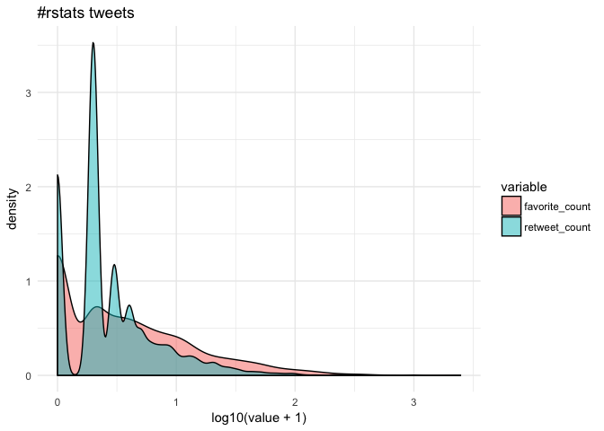
dim(rstats) [1] 2840 42Suppose our purpose is to foretell how well-liked tweets shall be primarily based on how typically the tweet was retweeted and favorited (which correlate strongly).
cor(rstats$favorite_count, rstats$retweet_count, methodology="spearman") [1] 0.7051952Since few tweeets go viral, the information are fairly skewed in the direction of zero.

Getting essentially the most out of formulation
Let’s suppose we’re concerned with placing tweets into classes primarily based on reputation however we’re undecided how finely-grained we wish to make distinctions. A few of the knowledge, like rstats$mentions_screen_name is available in a listing of various lengths, so let’s write a helper operate to depend non-NA entries.
Let’s begin with a dense neural web, the default of kms. We will use base R capabilities to assist clear the information–on this case, lower to discretize the result, grepl to search for key phrases, and weekdays and format to seize totally different points of the time the tweet was posted.
breaks <- c(-1, 0, 1, 10, 100, 1000, 10000)
reputation <- kms(lower(retweet_count + favorite_count, breaks) ~ screen_name +
                  supply + n(hashtags) + n(mentions_screen_name) +
                  n(urls_url) + nchar(textual content) +
                  grepl('picture', media_type) +
                  weekdays(created_at) +
                  format(created_at, '%H'), rstats)
plot(reputation$historical past)
  + ggtitle(paste("#rstat reputation:",
            paste0(spherical(100*reputation$evaluations$acc, 1), "%"),
            "out-of-sample accuracy"))
  + theme_minimal()

reputation$confusion
reputation$confusion

                    (-1,0] (0,1] (1,10] (10,100] (100,1e+03] (1e+03,1e+04]
      (-1,0]            37    12     28        2           0             0
      (0,1]             14    19     72        1           0             0
      (1,10]             6    11    187       30           0             0
      (10,100]           1     3     54       68           0             0
      (100,1e+03]        0     0      4       10           0             0
      (1e+03,1e+04]      0     0      0        1           0             0
The mannequin solely classifies about 55% of the out-of-sample knowledge accurately and that predictive accuracy doesn’t enhance after the primary ten epochs. The confusion matrix means that mannequin does finest with tweets which can be retweeted a handful of instances however overpredicts the 1-10 degree. The historical past plot additionally means that out-of-sample accuracy just isn’t very secure. We will simply change the breakpoints and variety of epochs.
breaks <- c(-1, 0, 1, 25, 50, 75, 100, 500, 1000, 10000)
reputation <- kms(lower(retweet_count + favorite_count, breaks) ~
                  n(hashtags) + n(mentions_screen_name) + n(urls_url) +
                  nchar(textual content) +
                  screen_name + supply +
                  grepl('picture', media_type) +
                  weekdays(created_at) +
                  format(created_at, '%H'), rstats, Nepochs = 10)

plot(reputation$historical past)
  + ggtitle(paste("#rstat reputation (new breakpoints):",
            paste0(spherical(100*reputation$evaluations$acc, 1), "%"),
            "out-of-sample accuracy"))
  + theme_minimal()
That helped some (about 5% extra predictive accuracy). Suppose we wish to add somewhat extra knowledge. Let’s first retailer the enter system.
pop_input <- "lower(retweet_count + favorite_count, breaks) ~
                          n(hashtags) + n(mentions_screen_name) + n(urls_url) +
                          nchar(textual content) +
                          screen_name + supply +
                          grepl('picture', media_type) +
                          weekdays(created_at) +
                          format(created_at, '%H')"
Right here we use paste0 so as to add to the system by looping over consumer IDs including one thing like:
grepl("12233344455556", mentions_user_id)mentions <- unlist(rstats$mentions_user_id)
mentions <- distinctive(mentions[which(table(mentions) > 5)]) # take away rare
mentions <- mentions[!is.na(mentions)] # drop NA
for(i in mentions)
pop_input <- paste0(pop_input, " + ", "grepl(", i, ", mentions_user_id)")
reputation <- kms(pop_input, rstats)
That helped a contact however the predictive accuracy remains to be pretty unstable throughout epochs…
Customizing layers with kms()
We might add extra knowledge, maybe add particular person phrases from the textual content or another abstract stat (imply(textual content %in% LETTERS) to see if all caps explains reputation). However let’s alter the neural web.
The enter.system is used to create a sparse mannequin matrix. For instance, rstats$supply (Twitter or Twitter-client utility sort) and rstats$screen_name are character vectors that shall be dummied out. What number of columns does it have?
[1] 1277Say we wished to reshape the layers to transition extra step by step from the enter form to the output.

kms builds a keras_sequential_model(), which is a stack of linear layers. The enter form is decided by the dimensionality of the mannequin matrix (reputation$P) however after that customers are free to find out the variety of layers and so forth. The kms argument layers expects a listing, the primary entry of which is a vector items with which to name keras::layer_dense(). The primary aspect the variety of items within the first layer, the second aspect for the second layer, and so forth (NA as the ultimate aspect connotes to auto-detect the ultimate variety of items primarily based on the noticed variety of outcomes). activation can be handed to layer_dense() and should take values equivalent to softmax, relu, elu, and linear. (kms additionally has a separate parameter to regulate the optimizer; by default kms(... optimizer="rms_prop").) The dropout that follows every dense layer fee prevents overfitting (however after all isn’t relevant to the ultimate layer).
Selecting a Batch Dimension
By default, kms makes use of batches of 32. Suppose we had been proud of our mannequin however didn’t have any specific instinct about what the dimensions needs to be.
Nbatch <- c(16, 32, 64)
Nruns <- 4
accuracy <- matrix(nrow = Nruns, ncol = size(Nbatch))
colnames(accuracy) <- paste0("Nbatch_", Nbatch)

est <- listing()
for(i in 1:Nruns){
  for(j in 1:size(Nbatch)){
   est[[i]] <- kms(pop_input, rstats, Nepochs = 2, batch_size = Nbatch[j])
   accuracy[i,j] <- est[[i]][["evaluations"]][["acc"]]
  }
}

colMeans(accuracy)
Nbatch_16 Nbatch_32 Nbatch_64
0.5088407 0.3820850 0.5556952 For the sake of curbing runtime, the variety of epochs was set arbitrarily quick however, from these outcomes, 64 is one of the best batch measurement.
Making predictions for brand new knowledge
So far, now we have been utilizing the default settings for kms which first splits knowledge into 80% coaching and 20% testing. Of the 80% coaching, a sure portion is put aside for validation and that’s what produces the epoch-by-epoch graphs of loss and accuracy. The 20% is barely used on the finish to evaluate predictive accuracy.
However suppose you wished to make predictions on a brand new knowledge set…
reputation <- kms(pop_input, rstats[1:1000,])
predictions <- predict(reputation, rstats[1001:2000,])
predictions$accuracy
[1] 0.579As a result of the system creates a dummy variable for every display title and point out, any given set of tweets is all however assured to have totally different columns. predict.kms_fit is an S3 methodology that takes the brand new knowledge and constructs a (sparse) mannequin matrix that preserves the unique construction of the coaching matrix. predict then returns the predictions together with a confusion matrix and accuracy rating.
In case your newdata has the identical noticed ranges of y and columns of x_train (the mannequin matrix), you too can use keras::predict_classes on object$mannequin.
Utilizing a compiled Keras mannequin
This part exhibits the best way to enter a mannequin compiled within the trend typical to library(keras), which is beneficial for extra superior fashions. Right here is an instance for lstm analogous to the imbd with Keras instance.
ok <- keras_model_sequential()
ok %>%
  layer_embedding(input_dim = reputation$P, output_dim = reputation$P) %>%
  layer_lstm(items = 512, dropout = 0.4, recurrent_dropout = 0.2) %>%
  layer_dense(items = 256, activation = "relu") %>%
  layer_dropout(0.3) %>%
  layer_dense(items = 8, # variety of ranges noticed on y (consequence)
              activation = 'sigmoid')

ok %>% compile(
  loss = 'categorical_crossentropy',
  optimizer = 'rmsprop',
  metrics = c('accuracy')
)

popularity_lstm <- kms(pop_input, rstats, ok)
Drop me a line by way of the challenge’s Github repo. Particular because of @dfalbel and @jjallaire for useful options!!